
From compute to clone: how we discover binders no one has made before
A visual walkthrough of the Ranomics integrated pipeline from computational protein design through experimental validation to confirmed binders
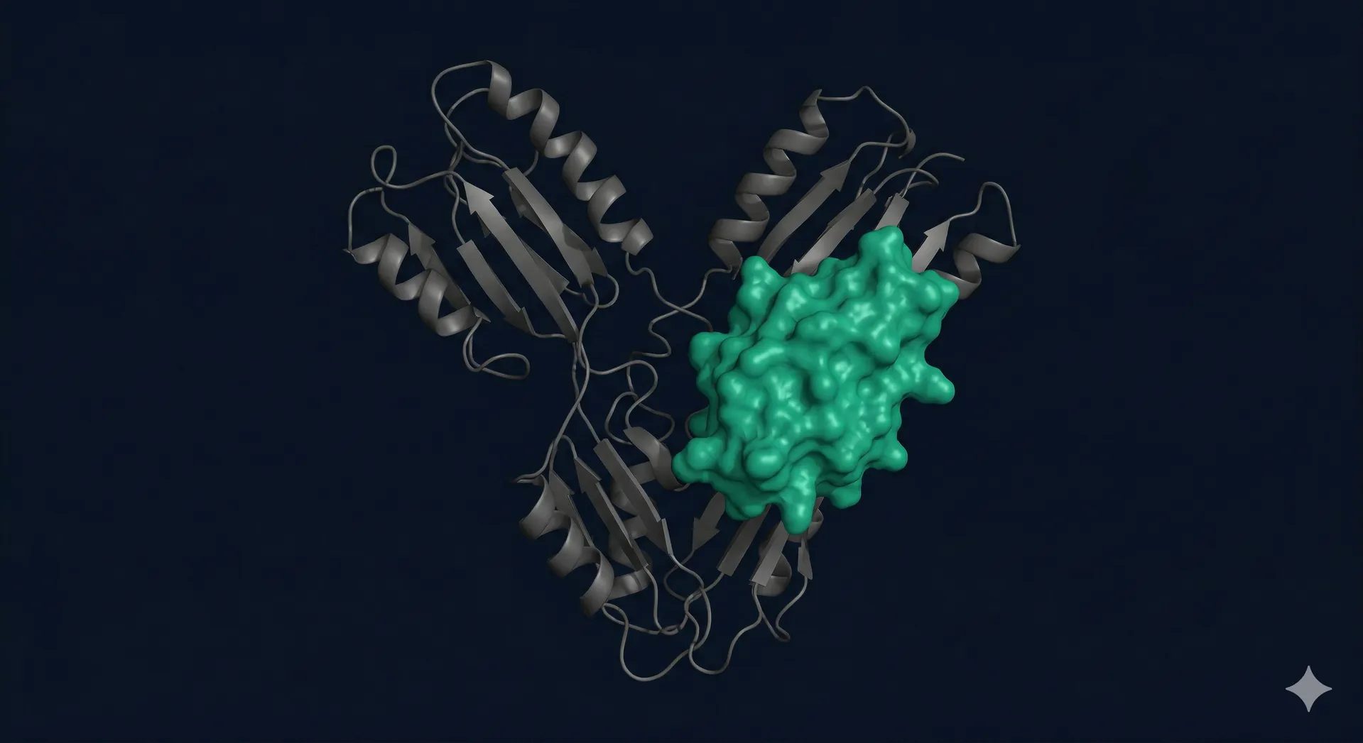
It starts with a structure, not a library
Traditional binder discovery starts with a library — a pool of sequences you hope contains something useful. The success of that approach depends entirely on whether your library happens to cover the right region of sequence space for your target.
Our approach starts with your target's three-dimensional structure. From that structure, we define the binding epitope and use it to constrain the design process computationally. The first step is knowing exactly where you want to bind — before generating a single sequence.
Library approach
Random sequence pool sampled from prior diversity. Hit rate depends on library coverage of relevant sequence space.
Design approach
Target structure + hotspot constraints drive scaffold generation. Every candidate is designed for the target.
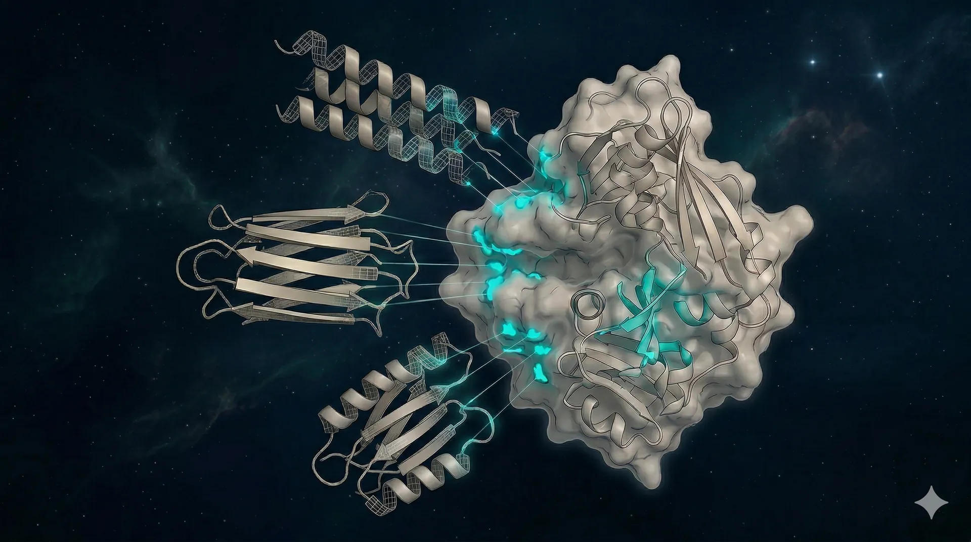
Three generative models design binder architectures in parallel
We run RFdiffusion, BindCraft, and Boltzgen in parallel — each model generates candidates suited to different scaffold types and binding geometries. RFdiffusion excels at hotspot-guided backbone generation. BindCraft iterates between scaffold generation, sequence design, and AlphaFold2 validation in a single loop. Boltzgen explores alternative backbone topologies via flow-based sampling.
ProteinMPNN and SolubleMPNN then assign amino acid sequences to each backbone, optimizing for stability, foldability, and solubility. The result is a combined candidate pool drawn from all three generators — the best candidates are selected regardless of which model produced them.
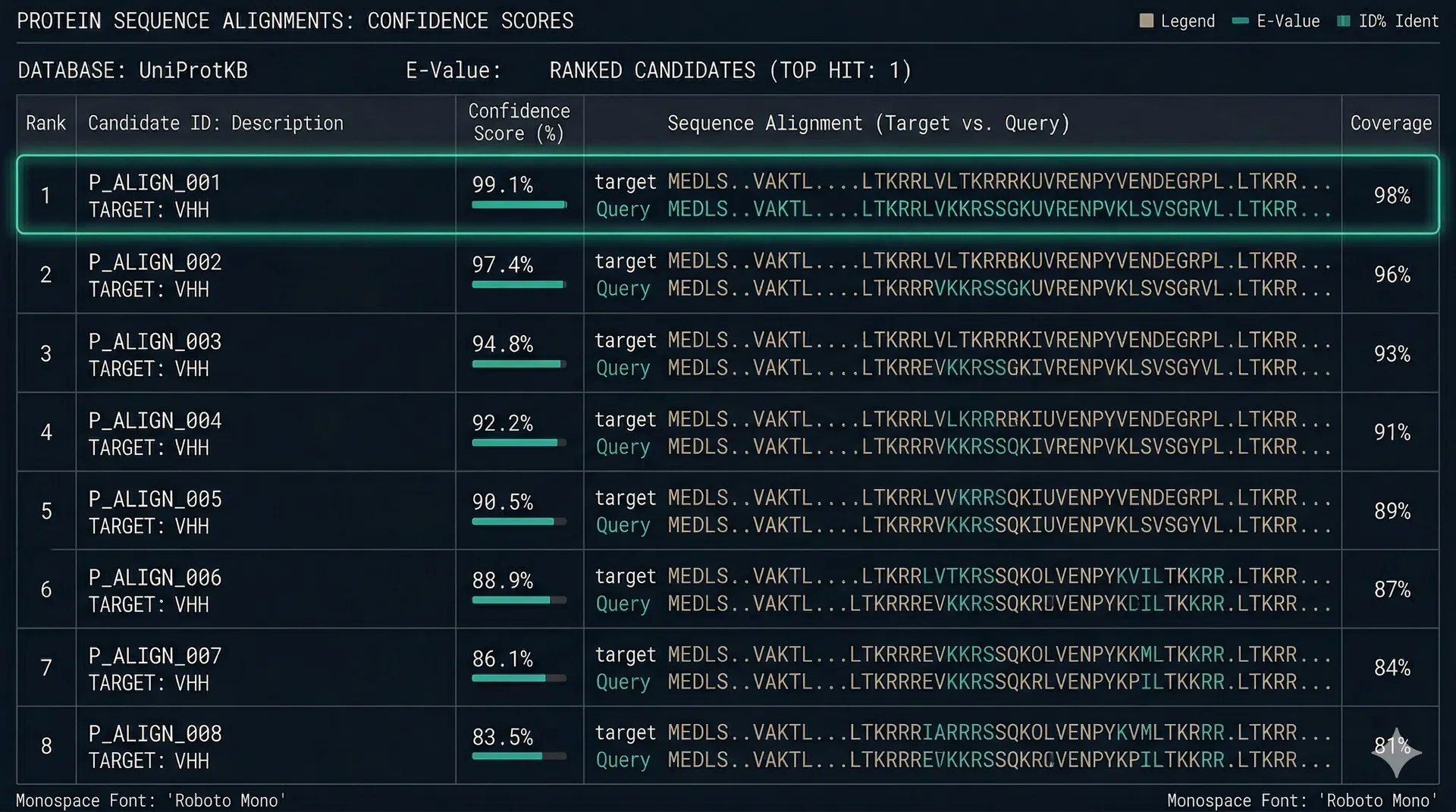
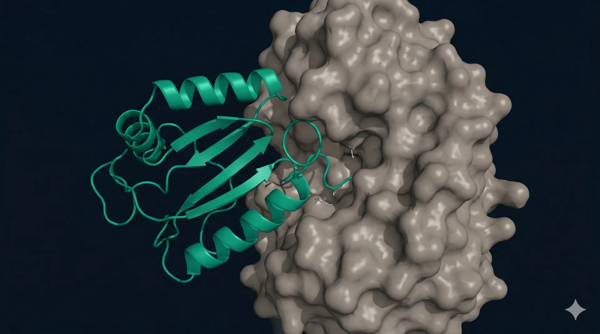
Structure prediction prunes the candidate pool
We use Boltz-2, ESMFold, and ColabFold (accelerated AlphaFold2) to predict the three-dimensional structure of each candidate in complex with the target. ESMFold provides rapid single-sequence fold checks, while Boltz-2 and ColabFold validate the full binder-target complex. Candidates that don't fold correctly, or whose predicted interface is weak, are removed before synthesis.
Filtering criteria are applied uniformly across all candidates regardless of which generative model produced them. Key metrics include interface pLDDT, predicted aligned error (PAE), ipTM, and solubility scores. The combined pool from all three generators is filtered down to the top candidates for wet-lab screening.
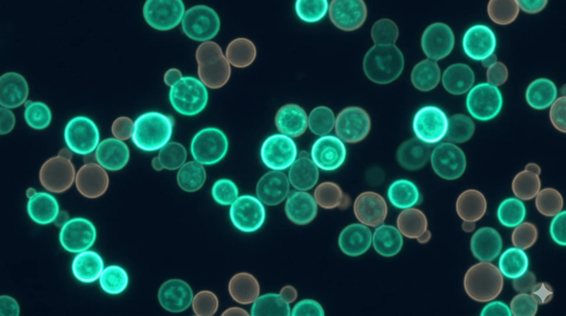
Filtered sequences become a screened library
The surviving computational candidates are synthesized as a pooled oligo library and cloned into a display construct. Each cell in the display population carries the gene encoding the binder it presents on its surface.
This genotype-phenotype linkage is what makes display screening work at scale: when we sort for binding cells, we can recover the sequence from the DNA inside, regardless of how many unique sequences are in the pool simultaneously.
Why display matters here. Display screening is not just a binding assay — it is a high-throughput enrichment that simultaneously evaluates thousands of sequences under identical conditions, without the parallelization overhead of individual protein expression and purification.
Display screening identifies real binders
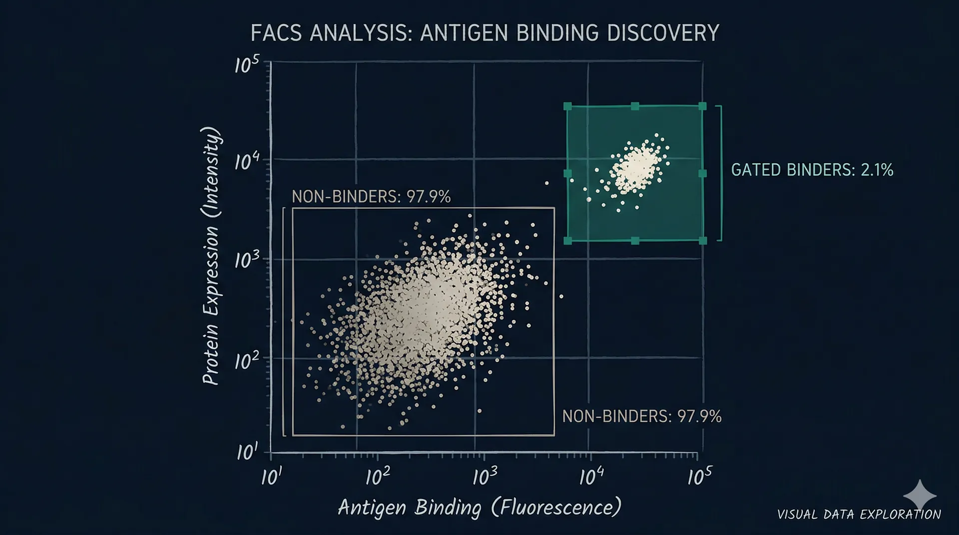
Cells displaying binders that engage a fluorescently labelled target are isolated using FACS or MACS. Selection stringency is calibrated to your affinity requirements — tighter gates select for higher-affinity binders at the cost of reducing the number of clones recovered.
Sorted populations are sequenced by NGS. We analyze enrichment of each unique sequence across the selected vs. unselected populations. Clones enriched by binding rather than by synthesis or display bias are identified and ranked.
Sequences that bind, not sequences that might
Every sequence in the final hit list has binding evidence from display. We do not deliver computational predictions as deliverables — the screen is the validation step, not optional.
From validated hits to lead candidates
Confirmed binders from the initial screen are the starting point for lead optimization. Affinity maturation through deep mutational scanning or focused library screening can improve binding kinetics by orders of magnitude. Stability and expression engineering ensure your lead candidates are developable.
The same display infrastructure used for the initial screen is used for maturation — the genotype-phenotype linkage, the NGS readout, and the selection stringency controls are already in place. No technology transition is required.
Pipeline questions
What does "compute to clone" mean? +
It describes the full pipeline from computational protein design (generating binder sequences on GPUs) through experimental validation (display screening, FACS selection) to delivering confirmed, sequence-verified clones. One team, one pipeline, no handoff between vendors.
How long does the full pipeline take? +
Our fixed-scope AI Binder Sprint runs 6-8 weeks end to end. Custom campaigns with additional design rounds, maturation, or extended screening may take longer. Timeline is specified at project start.
What is delivered at the end of the pipeline? +
Sequence-verified binder hits with binding evidence (display enrichment data, NGS analysis, and optionally BLI kinetics). Final deliverable includes ranked sequences, raw data, and a summary report.
Ready to run your own design campaign?
Tell us about your target. We will scope a binder discovery program and get back to you within 24 hours.